Methodology
Temporal logic control in a nutshell
Let us start with the linear temporal logic (LTL), a formalism that can specify high-level linear-time specifications and be operated by computer programs. An LTL formula defined over an alphabet, and it consists of propositional logic operators (logic 1: \(\top\), conjunction: \(\wedge\), and negation: \(\neg\)) and temporal operators (next \(\bigcirc\) and until \(\mathbf{U}\)).
An LTL formula is generated inductively according to the syntax in the Backus Naur form:
where \(p\) is an atomic proposition.
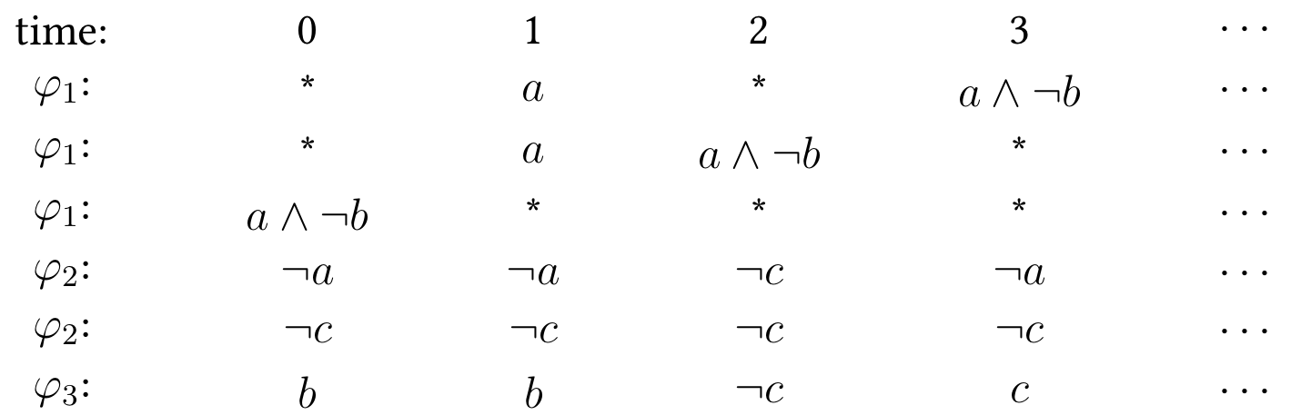
The semantics of LTL is defined on infinite words, i.e., infinite sequences of propositions \(\sigma_0\sigma_1\sigma_2\cdots\), over the alphabet \(2^{AP}\), where \(AP\) is a set of atomic propositions, and \(\sigma_i (i\in\mathbb{N})\) is a propositional formula.
Examples
Suppose that \(AP=\set{a,b,c}\). Then the following formulas
can be interpreted as
ROCS works with a very general form of dynamical systems
\(f:\,\mathbb{R}^n\times\mathbb{R}^m \to \mathbb{R}^n\): a Lipschitz continuous function,
\(\mathcal{X}\subset\mathbb{R}^n\): the non-empty compact state space,
\(\mathcal{U}\subset\mathbb{R}^m\): the non-empty and compact control space,
\(\mathcal{D}=\left\{d\in\mathbb{R}^n \mid \|d\|_\infty\leq\delta\right\} (\delta\geq 0)\): a set of perturbations.
To connect the LTL specification and the dynamics, ROCS asks for a labeling function \(L:\mathcal{X}\to 2^{AP}\), which associates properties to every state in the state space of a dynamical system. The labeling function \(L\) translates a solution of the dynamical system
into an infinite word (or trace) \(\text{Trace}(\mathbf{x})=\set{L(x_t)}_{t=0}^\infty\). If the system solution \(\mathbf{x}\) can be controlled such that \(\text{Trace}(\mathbf{x})\) satisfies a given LTL formula \(\varphi\), then \(\varphi\) is realizable for the system. The set of all initial conditions, from which a control strategy can realize \(\varphi\), is called the winning set of the system w.r.t. \(\varphi\).
A temporal logic control synthesis problem is to
determine whether a given LTL specification mathbf{x} is realizable for the system, and
synthesize a feedback control strategy such that the trace of any closed-loop system solution satisfies \(\varphi\) if possible.
There are two major frameworks for solving such a problem.
Abstraction-based Framework
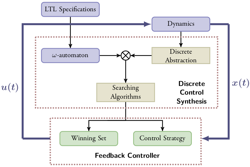
The framework of abstraction-based control consists of three steps:
Construct a finite transition system that over-approximates the original system behaviors, which is known as an abstraction.
Synthesize a discrete controller that satisfies the given specification over the finite abstraction if there exists one, otherwise returns empty. Such a discrete control synthesis is usually carried out by the algorithms for solving two-player infinite games over a product system of the abstraction and the specification. Usually, the LTL specifiation will be converted into a deterministic \(\omega\)-automaton first.
Translate the discrete controller into a continuous one that solves the original control synthesis problem.
Specification-guided Framwork
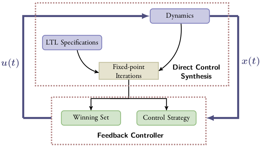
Unlike abstraction-based control, specification-guided control partitions the state space of the system incrementally with respect to both the dynamics and specification. The resulting partition of the state space is non-uniform. The Buechi game algorithm on a finite graph proceeds on the computation of the predecessors of a target set, which is the set of nodes that have out-going edges that point to the target set. Similarly for a dynamical system on a continuous state space, we can define the predecessor of a set of states \(X\subseteq\mathcal{X}\) as
and hence the Buechi game algorithm can be generalized to infinite-state systems. However, exactly computing the predecessors for the system is hard.
In ROCS, predecessors are inner-approximated by a union of intervals in the Paver by using an interval branch-and-bound scheme. Under this scheme, an interval is bisected only when it is undetermined to be contained inside a predecessor and its width is greater than a given precision \(\varepsilon\). Hence, the approximation error can be controlled by choosing a proper \(\varepsilon\). The Buechi game algorithm, as well as the specific algorithms for invariance, reachability, Buechi, and co-Buechi specifications, is implemented in the CSolver based on the data structure of the Paver.